Speeding up Bayesian sampling with map_rect
Fitting a full Bayesian model can be slow, especially with a large dataset. For example, it’d be great to analyse the climate crisis questions in the European Social Survey (ESS), which typically has around 45,000 respondents from around Europe on a range of socio-political questions. There are two main ways of parallelising your Bayesian model in Stan: between-chain parallelisation and within-chain parallelisation. The first of these is very easy to implement (chains = 4, cores = 4) - it simply runs the algorithm once on each core and pools the posterior samples at the end. The second method is more complicated as it requires a non-trivial modification to the Stan model, but can bring with it large speedups if you have the cores available. In this post we’ll get a >5x speedup of ordinal regression using within-chain parallelisation.
I’ll assume you are somewhat familiar with McElreath’s introduction with cmdstan, with Ignacio’s introduction with rstan, and/or with the Stan user guide. We’ll implement a mapped version of ordinal regression with one (factor) covariate using similar ideas. The main difference is that we’ll have a shard set up for each distinct level of the factor, and each shard will receive a different number of datapoints. This is my first attempt at making sense of this, so use at your own risk.
Important note: there is a bug in the ordered_logistic_lpmf function in stan 2.19.2, the version I currently have installed. Until the fixed version in stan 2.20, I went for the easy fix.
Setup
Suppose you have a large dataset and/or a log-likelihood function that is expensive to evaluate. Then you can break down your dataset into chunks (called shards), calculate the log-likelihood on each shard in parallel, then sum up the log-likelihood of each shard at the end.
There seem to be two types of within-chain parallelisation: threading and Message Passing Interface (MPI). MPI requires some extra setup and is typicaly used if you want to implement within-chain parallelisation across multiple computers. We’ll stick with the simpler threading method.
A thread is (confusingly) sometimes called a core. The number of threads you have will determine how many shards you can calculate at the same time. You can see how many threads you have available with nproc --all.
nproc --all4So I can run 4 threads at the same time. For a more detailed breakdown use lscpu, where the number of threads is given by CPU(s) and is equal to Thread(s) per core * Core(s) per socket * Socket(s). For me this is 4 = 1 * 4 * 1.
lscpuArchitecture: x86_64
CPU op-mode(s): 32-bit, 64-bit
Byte Order: Little Endian
CPU(s): 4
On-line CPU(s) list: 0-3
Thread(s) per core: 1
Core(s) per socket: 4
Socket(s): 1
NUMA node(s): 1
Vendor ID: GenuineIntel
CPU family: 6
Model: 158
Model name: Intel(R) Core(TM) i5-7600K CPU @ 3.80GHz
Stepping: 9
CPU MHz: 3993.031
CPU max MHz: 4200,0000
CPU min MHz: 800,0000
BogoMIPS: 7584.00
Virtualisation: VT-x
L1d cache: 32K
L1i cache: 32K
L2 cache: 256K
L3 cache: 6144K
NUMA node0 CPU(s): 0-3
Flags: fpu vme de pse tsc msr pae mce cx8 apic sep mtrr pge mca cmov pat pse36 clflush dts acpi mmx fxsr sse sse2 ss ht tm pbe syscall nx pdpe1gb rdtscp lm constant_tsc art arch_perfmon pebs bts rep_good nopl xtopology nonstop_tsc cpuid aperfmperf tsc_known_freq pni pclmulqdq dtes64 monitor ds_cpl vmx est tm2 ssse3 sdbg fma cx16 xtpr pdcm pcid sse4_1 sse4_2 x2apic movbe popcnt tsc_deadline_timer aes xsave avx f16c rdrand lahf_lm abm 3dnowprefetch cpuid_fault invpcid_single pti ssbd ibrs ibpb stibp tpr_shadow vnmi flexpriority ept vpid fsgsbase tsc_adjust bmi1 hle avx2 smep bmi2 erms invpcid rtm mpx rdseed adx smap clflushopt intel_pt xsaveopt xsavec xgetbv1 xsaves dtherm ida arat pln pts hwp hwp_notify hwp_act_window hwp_epp md_clear flush_l1dBefore compiling a model with threading, we have to tell Stan to compile with threading. For me, this worked by adding -DSTAN_THREADS -pthread to my Makevars file. Check out the recommendations in the docs for more information on this.
Sys.getenv("HOME") %>%
  file.path(".R", "Makevars") %>%
  print() %>%
  read_file() %>%
  writeLines()
[1] "/home/brian/.R/Makevars"
CXX14FLAGS = -O3 -march=native -mtune=native
CXX14FLAGS += -fPIC
CXX14FLAGS += -DSTAN_THREADS
CXX14FLAGS += -pthreadBefore fitting a model with threading, we’ll have to tell Stan how many threads are available via the environment variable STAN_NUM_THREADS. We’ll run it now just to be sure.
Sys.setenv(STAN_NUM_THREADS = 4)Now we’re all setup for threading.
Generate the data
Let’s generate observations from the prior predictive distribution. Skip this section if you’re just interested in the parallelisation. We’ll a similar model as described in Michael Betancourt’s case study. The main difference is that we’ll use contrast factors for our latent effect.
m_sim <- "models/ordinal_regression_sim_betancourt.stan" %>%
  here() %>%
  stan_model()
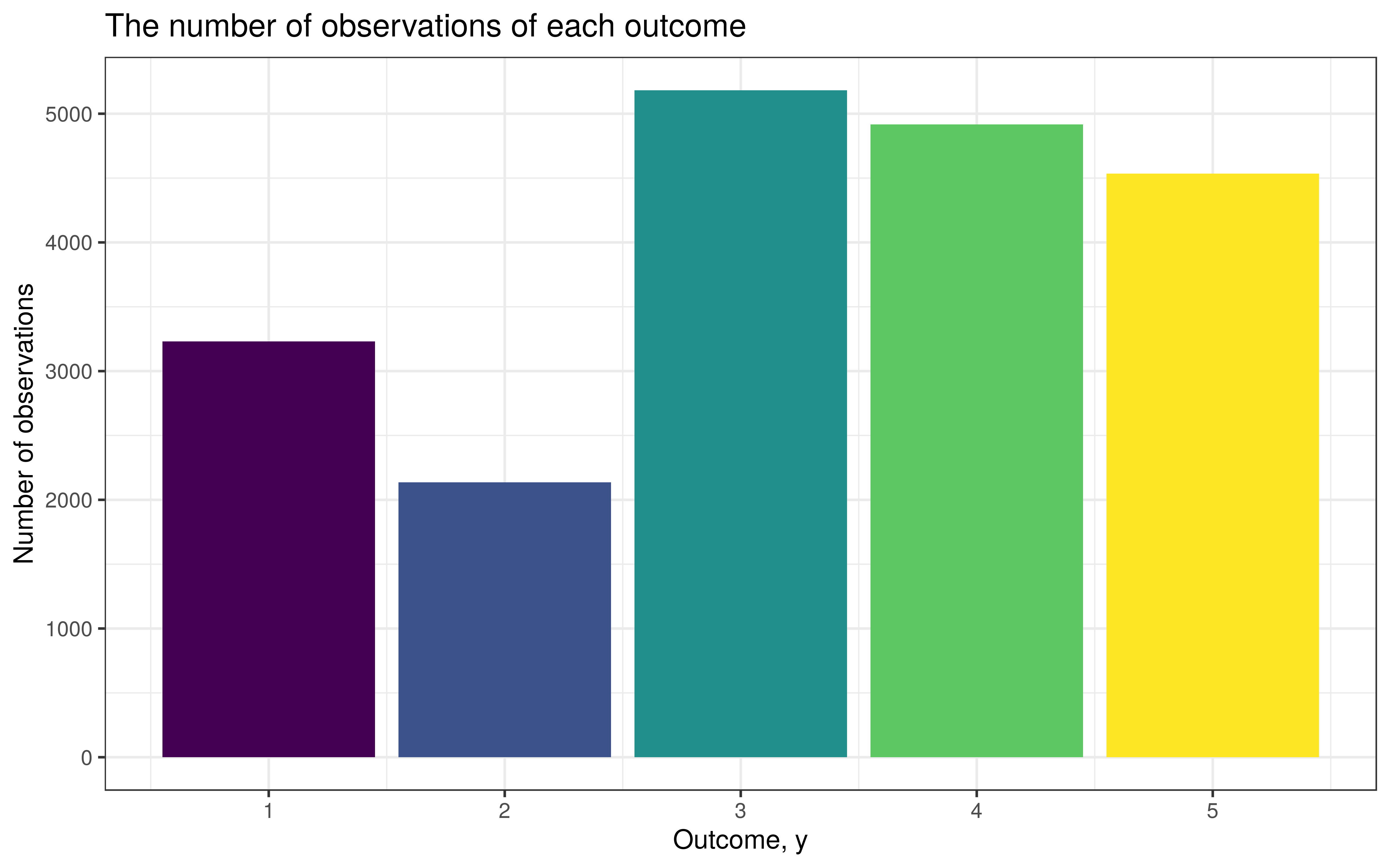
We’ll generate 20,000 observations, where the only covariate is called factr, of which we have around 50 unique values. Notice that we will end up with a different number of observations for each level of factr.
set.seed(12096)

N <- 20000 # number of observations
K <- 5     # number of ordinal outcomes
L <- 50    # number of unique levels in our factor

# the covariates
df_sim <- 1:L %>%
  sample(size = N, replace = TRUE) %>%
  tibble(factr = .) %>%
  mutate(factr = factr %>% as_factor() %>% fct_reorder(factr)) %>%
  arrange(factr)

# in list-format for stan
data_sim <- list(
  N = N,
  K = K,
  L = L,
  factr = model.matrix(~ 1 + factr, df_sim)[, 2:L], # contrast encoding
  # hyperparameters
  factr_mu = 0,
  factr_sd = 1,
  alpha = c(2, 4, 8, 4, 2)
)
Now we simply draw once from the prior predictive distribution, then extract the parameters and outcome.
# draw from the prior predictive distribution
fit_sim <- m_sim %>%
  sampling(
    algorithm = 'Fixed_param',
    data = data_sim,
    iter = 1,
    chains = 1,
    seed = 43484
  )

# extract the parameters and observations
cutpoints <- fit_sim %>%
  spread_draws(c[i]) %>%
  pull(c)

effects <- fit_sim %>%
  spread_draws(beta[i]) %>%
  pull(beta)

y <- fit_sim %>%
  spread_draws(y[i]) %>%
  pull(y)

# put covariates and outcome in the one dataset
df <- df_sim %>%
  mutate(
    y = y,
    factr = factr %>% as.integer()
  ) %>%
  arrange(factr)

# as a list for stan
data <- data_sim %>%
  list_modify(y = df$y)
The unmapped model
Let’s check that Betancourt’s model m passes some standard diagnostic tests on our data and time how long it takes to fit.
m <- "models/ordinal_regression_betancourt.stan" %>%
  here() %>%
  stan_model()
start <- Sys.time()
fit <- m %>%
sampling(
data = data,
chains = 1,
warmup = 500,
iter = 2000,
seed = 14031
)
end <- Sys.time()
duration <- end - startThe fitting took 5.7 minutes.
The HMC diagnostics look good.
rstan::check_hmc_diagnostics(fit)Divergences:
0 of 1500 iterations ended with a divergence.
Tree depth:
0 of 1500 iterations saturated the maximum tree depth of 10.
Energy:
E-BFMI indicated no pathological behavior.The rhat is smaller than 1.05 and the bulk/tail ESS are over 100, which is good.
| variable | rhat_min | ess_bulk_min | ess_tail_min | rhat_max | ess_bulk_max | ess_tail_max |
|---|---|---|---|---|---|---|
| beta | 1.00 | 165.98 | 306.02 | 1.01 | 254.76 | 654.57 |
| c | 1.01 | 102.99 | 179.38 | 1.01 | 107.56 | 214.77 |
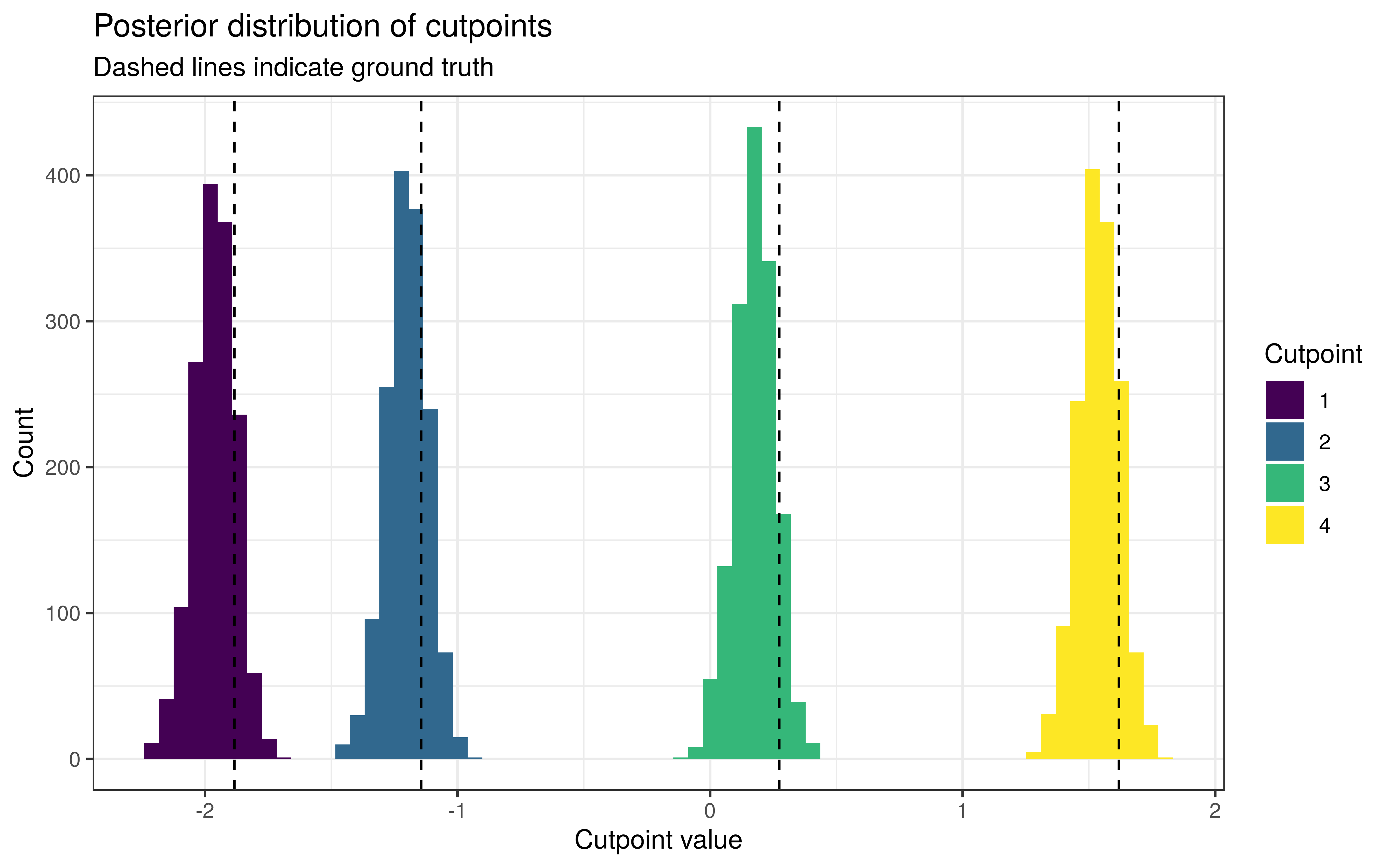
The cutpoints have been estimated slightly too low, but within reasonable bounds.

Around 93.9% of the 90% intervals for β contained the true values. This is not bad considering that one error carries the weight of over 2 percentage points.
The mapped model
Now for the mapped version.
m_mapped <- "models/ordinal_regression_mapped.stan" %>%
  here() %>%
  stan_model()
We’ll set up a shard for every level of our factor. The function lp for calculating the log-posterior on one shard looks like this. The first entry in our integer array xi is the number of observations M for this level/shard. The data we need is then contained in the next M entries of xi. The cutpoints are the only global parameters we’ll use here. The estimated effect for this level is given by beta, the only local parameter for this shard. The log-likelihood ll is then calculated as usual.
functions {
  vector lp(vector global, vector local, real[] xr, int[] xi) {
    int M = xi[1];
    int y[M] = xi[2:M+1];
    vector[4] c = global[1:4];
    real beta = local[1];

    real ll = ordered_logistic_lpmf(y | rep_vector(beta, M), c);

    return [ll]';
  }
}
The shards are set up in the transformed data section. Since we have a shard for every level, we simply index the shards using the levels. This makes it very easy to keep track of which shard gets the next datapoint. The first entry of each shard is reserved for the number of datapoints used in that shard. To keep track of where to put the next datapoint within a shard, we setup the array j. This starts at 2 because position 1 is reserved for the number of datapoints in the shard. Everytime we add a datapoint to a shard, we increment that shard’s entry in j so that the next datapoint lands in the correct place.
transformed data {
  int<lower = 0, upper = N> counts[L] = count(factr, L);

  int<lower = 1> M = max(counts) + 1;

  int xi[L, max(counts) + 1];
  real xr[L, max(counts) + 1];

  int<lower = 1> j[L] = rep_array(2, L);
  xi[, 1] = counts;
  for (i in 1:N) {
    int shard = factr[i];
    xi[shard, j[shard]] = y[i];
    j[shard] += 1;
  }
}
I really like this way of creating shards because it doesn’t become such a mess of indices.
Now let’s time it.
start_mapped <- Sys.time()

fit_mapped <- m_mapped %>%
  sampling(
    data = data %>% list_modify(factr = df$factr),
    chains = 1,
    warmup = 500,
    iter = 2000,
    seed = 98176
  )

end_mapped <- Sys.time()
duration_mapped <- end_mapped - start_mapped
The fitting took 64.8523884 seconds. This is a 5.3-fold speedup!
The HMC diagnostics look good.
rstan::check_hmc_diagnostics(fit_mapped)Divergences:
0 of 1500 iterations ended with a divergence.
Tree depth:
0 of 1500 iterations saturated the maximum tree depth of 10.
Energy:
E-BFMI indicated no pathological behavior.The rhat and ESS values are still good.
| variable | rhat_min | ess_bulk_min | ess_tail_min | rhat_max | ess_bulk_max | ess_tail_max |
|---|---|---|---|---|---|---|
| beta | 0.999 | 439.148 | 587.322 | 1.005 | 634.109 | 979.157 |
| c | 1.001 | 286.037 | 422.349 | 1.003 | 293.793 | 481.067 |
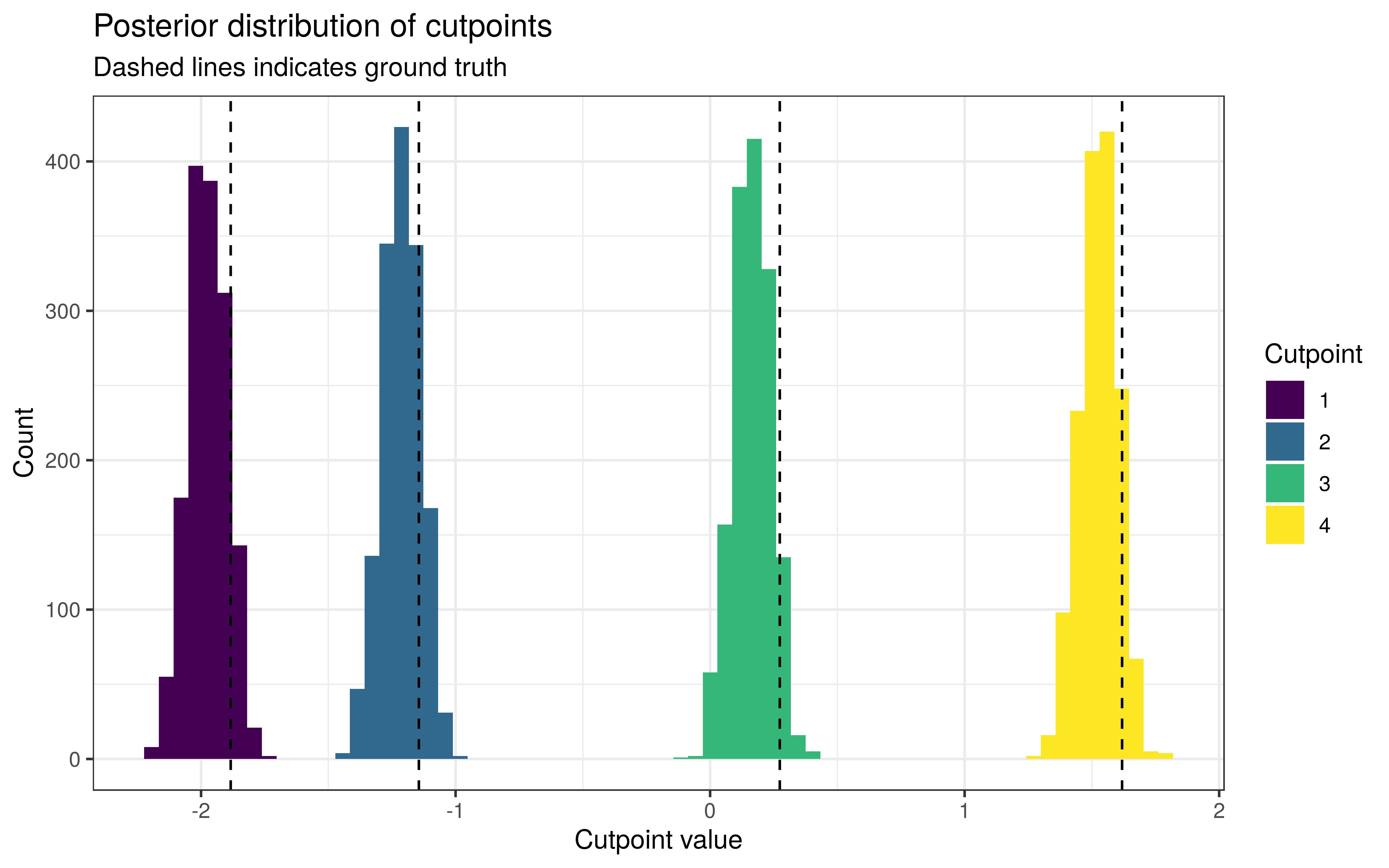
The posteriors of the cutpoints are much the same as before.

The level-effects are as well-calibrated as before, with around 93.9% of the 90% intervals for β containing the true values.
We can measure the similarity of the estimates in two ways:
- the absolute difference in the point estimates; and
- the ratio between the length of the overlap of the two 90% intervals and the length of the shortest of the two 90% intervals.
In each case the estimates look roughly the same, especially with respect to the ratio metric. The differences are a bit larger than I would have expected, but I’m not so sure on what scale a ‘good’ difference would be.
| metric | value |
|---|---|
| change_max | 0.0153 |
| change_mean | 0.0102 |
| change_median | 0.0107 |
| change_min | 0.0032 |
| ratio_max | 1.0000 |
| ratio_mean | 0.9897 |
| ratio_median | 0.9960 |
| ratio_min | 0.9619 |
Next steps
I’m fairly happy with the speedup seen here. Actually, I’m mostly happy I got it working at all. It’s entirely possible that creating 50 shards with only 4 threads to run them on isn’t the most efficient way to use threading, but I’ll keep doing it like this until there’s a more convenient way to do it. Higher up in my priorities right now are:
- adding more covariates, especially factors; and
- putting a hierarchical prior on the factor; e.g. for use in MRP.
The bulk ESS values are a bit on the low side, so there could be a better way to parameterise the model.